2. Markov Decision Process

The Markov Decision Process () is the core problem model of reinforcement learning. Whether you are training a quadruped robot to walk or having a robotic arm complete a grasping task, the first step is always to model the problem as an MDP — specifying the state space, action space, state transition probabilities, reward function, and other elements.

Embodied AI Perspective: Taking robotic arm grasping as an example, the state can be the joint angles plus the object's pose, the action is the target torque for each joint, and the reward signals whether the grasp succeeded. Once these elements are defined, RL algorithms can be used to solve for the optimal policy.

2.1 Agent–Environment Interaction

As shown below, the agent () interacts with the environment () over a series of discrete time steps. At each time step , the agent receives the environment state and selects an action based on that state. After executing the action, the agent receives a reward , and the environment transitions to the next state .

Agent–environment interaction process

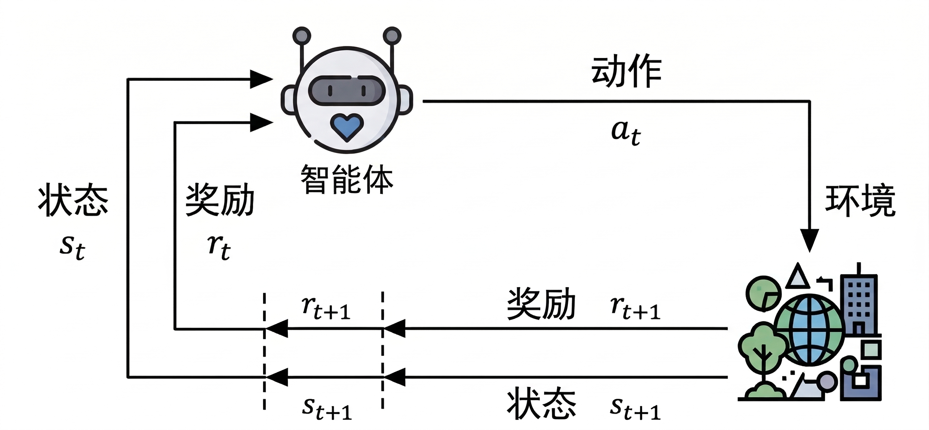
This process repeats continuously, forming a trajectory:

Completing a full trajectory (from the initial state to a terminal state) is called an episode, typically ending after a finite number of time steps .

To solve a problem with reinforcement learning, the first step is to model it as a Markov Decision Process — explicitly defining the state space, action space, state transition probabilities, and reward function. An MDP is usually defined by a five-tuple:

Here is the state space, is the action space, is the state transition probability matrix, is the reward function, and is the discount factor (with values in ).

2.2 The Markov Property

The core assumption of a Markov Decision Process is the Markov property: the probability distribution of future states depends only on the current state and action, and is independent of past states and actions:

In real robot scenarios, the Markov property is rarely satisfied strictly. For example, in robot navigation, the current LiDAR scan may not fully describe the environment state (due to occlusion). In most cases, however, an appropriate state representation (such as stacking historical frames) can approximate the Markov property. Such a process is called a Partially Observable Markov Decision Process (POMDP).

2.3 State Transition Matrix

For a finite state space, transitions between states can be represented by a state-flow diagram, as shown below:

Markov chain

The probability of switching between states can be written as a matrix:

Here is the number of states, and the transition probabilities from any given state to all other states sum to . The state transition matrix is part of the environment, describing how environment states evolve.

2.4 Goal and Return

The agent's goal is to interact with the environment and learn an optimal policy so that the actions selected in each state maximize the accumulated reward. This accumulated reward is called the return:

The discount factor controls how important future rewards are in the current decision. When is close to , the agent focuses on immediate rewards; when is close to , it places greater weight on future rewards.

The discount factor can also be used to quantify how far ahead the agent looks, known as the effective horizon:

When , , meaning the agent cares about rewards within roughly the next time steps. For tasks like robot locomotion, a relatively large is typically needed to account for long-term motion stability.

Recursive definition of the return:

2.5 Policy and Value

2.5.1 Policy

A policy () is the rule the agent uses to select actions in each state, denoted by :

A policy can be deterministic (always selecting the same action in a given state) or stochastic (selecting actions according to a probability distribution). In embodied AI, stochastic policies are more common because they provide better exploration and robustness.

2.5.2 State Value

The state value function gives the expected return when, starting from a given state, decisions are made according to policy :

2.5.3 Action Value

The action value function gives the expected return for taking action in state :

2.5.4 Relationship Between State Value and Action Value

The state value is a weighted average over all possible action values. State value reflects how good the policy itself is, while action value more specifically reflects how good it is to choose a particular action in a given state.

2.6 Model-Based vs. Model-Free

• Model-Based: Uses an environment model (state transition probabilities and reward function) for planning and decision-making, such as dynamic programming. In simulation environments, an environment model is sometimes available to accelerate learning.
• Model-Free: Does not rely on an environment model; learns directly through interaction with the environment, such as PPO and SAC. These methods are more widely used in real robot scenarios, because the dynamics of the real world are usually hard to obtain precisely.

2.7 Prediction vs. Control

• Prediction: Given a fixed policy, evaluate how good the policy is — i.e., compute its value function.
• Control: Find an optimal policy that maximizes the accumulated return.

In complex problems, prediction and control typically need to be addressed jointly — evaluating the current policy while learning an optimal one. This is precisely the idea behind the Actor-Critic framework.